Hessian matrix
In mathematics, the Hessian matrix (or simply the Hessian) is the square matrix of second-order partial derivatives of a function; that is, it describes the local curvature of a function of many variables. The Hessian matrix was developed in the 19th century by the German mathematician Ludwig Otto Hesse and later named after him. Hesse himself had used the term "functional determinants".
Given the real-valued function
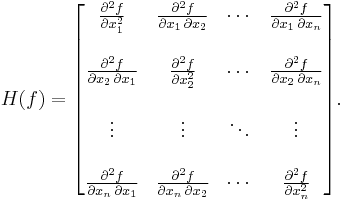
if all second partial derivatives of f exist, then the Hessian matrix of f is the matrix
where x = (x1, x2, ..., xn) and Di is the differentiation operator with respect to the ith argument and the Hessian becomes
Because f is often clear from context,  is frequently shortened to simply
  .
.
Some mathematicians[1] define the Hessian as the determinant of the above matrix.
Hessian matrices are used in large-scale optimization problems within Newton-type methods because they are the coefficient of the quadratic term of a local Taylor expansion of a function. That is,
where J is the Jacobian matrix, which is a vector (the gradient for scalar-valued functions). The full Hessian matrix can be difficult to compute in practice; in such situations, quasi-Newton algorithms have been developed that use approximations to the Hessian. The best-known quasi-Newton algorithm is the BFGS algorithm.
Contents |
Mixed derivatives and symmetry of the Hessian
The mixed derivatives of f are the entries off the main diagonal in the Hessian. Assuming that they are continuous, the order of differentiation does not matter (Clairaut's theorem). For example,
This can also be written as:
In a formal statement: if the second derivatives of f are all continuous in a neighborhood D, then the Hessian of f is a symmetric matrix throughout D; see symmetry of second derivatives.
Critical points and discriminant
If the gradient of f (i.e., its derivative in the vector sense) is zero at some point x, then f has a critical point (or stationary point) at x. The determinant of the Hessian at x is then called the discriminant. If this determinant is zero then x is called a degenerate critical point of f, this is also called a non-Morse critical point of f. Otherwise it is non-degenerate, this is called a Morse critical point of f.
Second derivative test
The following test can be applied at a non-degenerate critical point x. If the Hessian is positive definite at x, then f attains a local minimum at x. If the Hessian is negative definite at x, then f attains a local maximum at x. If the Hessian has both positive and negative eigenvalues then x is a saddle point for f (this is true even if x is degenerate). Otherwise the test is inconclusive.
Note that for positive semidefinite and negative semidefinite Hessians the test is inconclusive (yet a conclusion can be made that f is locally convex or concave respectively). However, more can be said from the point of view of Morse theory.
In view of what has just been said, the second derivative test for functions of one and two variables is simple. In one variable, the Hessian contains just one second derivative; if it is positive then x is a local minimum, if it is negative then x is a local maximum; if it is zero then the test is inconclusive. In two variables, the determinant can be used, because the determinant is the product of the eigenvalues. If it is positive then the eigenvalues are both positive, or both negative. If it is negative then the two eigenvalues have different signs. If it is zero, then the second derivative test is inconclusive.
Bordered Hessian
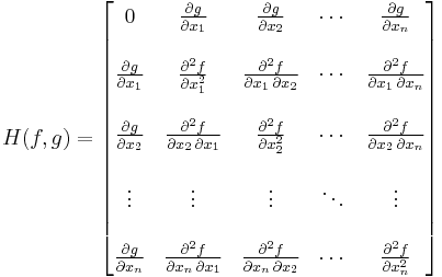
A bordered Hessian is used for the second-derivative test in certain constrained optimization problems. Given the function as before:
but adding a constraint function such that:
the bordered Hessian appears as
If there are, say, m constraints then the zero in the north-west corner is an m × m block of zeroes, and there are m border rows at the top and m border columns at the left.
The above rules of positive definite and negative definite can not apply here since a bordered Hessian can not be definite: we have z'Hz = 0 if vector z has a non-zero as its first element, followed by zeroes.
The second derivative test consists here of sign restrictions of the determinants of a certain set of n - m submatrices of the bordered Hessian.[2] Intuitively, think of the m constraints as reducing the problem to one with n - m free variables. (For example, the maximization of  subject to the constraint
  can be reduced to the maximization of
  without constraint.)
Vector-valued functions
If f is instead a function from  , i.e.
then the array of second partial derivatives is not a two-dimensional matrix of size  , but rather a tensor of order 3. This can be thought of as a multi-dimensional array with dimensions
  , which degenerates to the usual Hessian matrix for
  .
.
Generalizations to Riemannian manifolds
Let  be a Riemannian manifold and
  its Levi-Civita connection. Let
  be a smooth function. We may define the Hessian tensor
 by
by  ,
,
where we have taken advantage of the first covariant derivative of a function being the same as ordinary derivative. Choosing local coordinates  we obtain the local expression for the Hessian as
where  are the Christoffel symbols of the connection. Other equivalent forms for the Hessian are given by
 and
and  .
.
See also
- The determinant of the Hessian matrix is a covariant; see Invariant of a binary form
- Jacobian matrix
- The Hessian matrix is commonly used for expressing image processing operators in image processing and computer vision (see the Laplacian of Gaussian (LoG) blob detector, the determinant of Hessian (DoH) blob detector and scale space).
Notes
- ^ For instance, Binmore & Davies, (2007), Calculus Concepts and Methods, Cambridge University Press, p.190.
- ^ Neudecker, Heinz; Magnus, Jan R. (1988), Matrix differential calculus with applications in statistics and econometrics, New York: John Wiley & Sons, ISBN 978-0-471-91516-4, page 136


